UPSC 2026 Maths Optional Paper 2 Q1e — Step-by-Step Solution

10 marks · Section A

Duality · Linear Programming · asked 5× in 14 yrs · Read the full method →

Question

Solve the dual problem of the following linear programming problem by the graphical method:

Minimize $Y = 10y_1 + 6y_2 + 2y_3 + y_4$

subject to the constraints:

y_1 + y_2 + y_3 + y_4 \geq 2

2y_1 + y_2 - y_3 - 2y_4 \geq 1

y_1,\, y_2,\, y_3,\, y_4 \geq 0

Technique

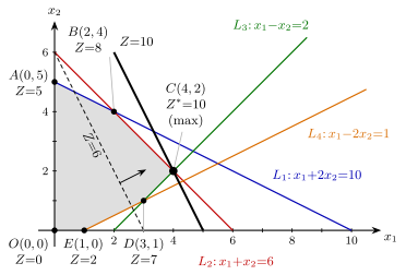
The printed problem has four variables, so it cannot be drawn; but it has only two constraints, so its dual has two variables and can be drawn. That asymmetry is the entire point of the question — the examiner is testing whether the candidate sees that dualising is a device for reducing dimension, not a formality. The printed problem is already in canonical minimisation form ( $\min c^{T}y$ , $Ay\ge b$ , $y\ge0$ ), whose dual is the maximisation $\max b^{T}x$ , $A^{T}x\le c$ , $x\ge0$ : four $\le$ constraints in two non-negative variables, solved by the corner-point method. Finally, since the question is posed about the printed primal, a complete answer returns from the dual to the primal by strong duality ( $Y^{*}=Z^{*}$ ) and complementary slackness (which recovers $y^{*}$ itself).

Solution

Step 1 — Put the printed problem in canonical form and name the data.

The printed (primal) problem is

\text{(P)}\qquad \min\ Y=c^{T}y \quad\text{s.t.}\quad Ay\ \ge\ b,\qquad y\ge 0,

with

c=\begin{pmatrix}10\\6\\2\\1\end{pmatrix},\qquad A=\begin{pmatrix}1&1&1&1\\[2pt]2&1&-1&-2\end{pmatrix},\qquad b=\begin{pmatrix}2\\1\end{pmatrix},\qquad y=\begin{pmatrix}y_1\\y_2\\y_3\\y_4\end{pmatrix}.

It is a minimisation with all constraints $\ge$ and all variables $\ge0$ — i.e. already in the canonical form for which the duality rules apply directly, with no need to reverse any inequality or split any variable.

Step 2 — Construct the dual, and derive it rather than merely quote it.

Assign a dual variable $x_1\ge0$ to the first constraint and $x_2\ge0$ to the second. Multiplying the constraints by these non-negative numbers preserves the inequalities; adding,

x_1\big(y_1+y_2+y_3+y_4\big)+x_2\big(2y_1+y_2-y_3-2y_4\big)\ \ge\ 2x_1+x_2 .

Regroup the left side by columns of $A$ , i.e. by the $y_j$ :

y_1(x_1+2x_2)+y_2(x_1+x_2)+y_3(x_1-x_2)+y_4(x_1-2x_2)\ \ge\ 2x_1+x_2 .

Now if the coefficient of each $y_j$ is held below the corresponding cost $c_j$ , then since every $y_j\ge0$ the left side is at most $10y_1+6y_2+2y_3+y_4=Y$ , and we obtain the bound $Y\ge 2x_1+x_2$ . This forces exactly the following requirements, and gives weak duality for free:

\text{(D)}\qquad \max\ Z=2x_1+x_2

\text{subject to}\qquad \begin{aligned} L_1:&\quad x_1+2x_2\ \le\ 10 &&(\text{from the } y_1\text{ column})\\ L_2:&\quad x_1+\ \ x_2\ \le\ 6 &&(\text{from the } y_2\text{ column})\\ L_3:&\quad x_1-\ \ x_2\ \le\ 2 &&(\text{from the } y_3\text{ column})\\ L_4:&\quad x_1-2x_2\ \le\ 1 &&(\text{from the } y_4\text{ column})\\ &\quad x_1,\ x_2\ \ge\ 0 . \end{aligned}

Equivalently, in matrix form, $\max b^{T}x$ subject to $A^{T}x\le c$ , $x\ge0$ — the rows of $A^{T}$ being the columns of $A$ , and the cost vector of the dual being the right-hand side $b$ of the primal.

(Recorded for Step 7: the derivation above proves $Z\le Y$ for every feasible pair $(x,y)$ — weak duality — so any feasible $x$ with $Z=Y$ for some feasible $y$ certifies optimality of both.)

(D) has two variables and is what the question asks us to solve graphically.

Step 3 — The graph: what to draw.

Work in the first quadrant of the $(x_1,x_2)$ -plane, $0\le x_1\le 11$ , $0\le x_2\le 6$ . Draw each constraint as its boundary line and shade the side containing the origin (the origin satisfies all four, since $0\le10,\,0\le6,\,0\le2,\,0\le1$ ):

Line	Equation	Two convenient points to join	Half-plane retained
$L_1$	$x_1+2x_2=10$	$(10,0)$ and $(0,5)$	below/left (origin side)
$L_2$	$x_1+x_2=6$	$(6,0)$ and $(0,6)$	below/left (origin side)
$L_3$	$x_1-x_2=2$	$(2,0)$ and $(4,2)$	above/left (origin side)
$L_4$	$x_1-2x_2=1$	$(1,0)$ and $(3,1)$	above/left (origin side)

( $L_3$ and $L_4$ meet the $x_2$ -axis at $(0,-2)$ and $(0,-\tfrac12)$ , outside the quadrant, so plot each through the two first-quadrant points listed.)

The feasible region is the convex polygon

O(0,0)\ \to\ E(1,0)\ \to\ D(3,1)\ \to\ C(4,2)\ \to\ B(2,4)\ \to\ A(0,5)\ \to\ O,

traversed anticlockwise, whose six edges lie on $x_2=0$ (from $O$ to $E$ ), $L_4$ ( $E$ to $D$ ), $L_3$ ( $D$ to $C$ ), $L_2$ ( $C$ to $B$ ), $L_1$ ( $B$ to $A$ ) and $x_1=0$ ( $A$ to $O$ ). Every constraint supports an edge, so no constraint is redundant. The region is non-empty (it contains $O$ ) and bounded (it lies in $0\le x_1\le6$ , $0\le x_2\le5$ ), so by the fundamental theorem of linear programming an optimal solution exists and is attained at a vertex.

Finally superimpose one iso-profit line $2x_1+x_2=k$ , e.g. $k=6$ through $(3,0)$ and $(0,6)$ , of slope $-2$ , and translate it parallel to itself away from the origin; label the last vertex it touches.

$Graphical solution of the dual in the (x_1,x_2)-plane, window 0\le x_1\le 10.5, 0\le x_2\le 6.5. The four constraint boundaries are drawn right across the window and labelled: L_1: x_1+2x_2=10 (blue, through (10,0) and (0,5)); L_2: x_1+x_2=6 (red, through (6,0) and (0,6)); L_3: x_1-x_2=2 (green, through (2,0) and (4,2)); and L_4: x_1-2x_2=1 (orange, through (1,0) and (3,1)) — the last two have negative x_2-intercepts and are plotted through their first-quadrant points. The feasible region is the shaded convex hexagon O(0,0)\to E(1,0)\to D(3,1)\to C(4,2)\to B(2,4)\to A(0,5)\to O, whose six edges lie on x_2=0, L_4, L_3, L_2, L_1 and x_1=0 respectively, so every constraint supports exactly one edge and none is redundant. Each vertex carries a dot and its coordinates with the objective value: O(0,0), Z=0; E(1,0), Z=2; D(3,1), Z=7; C(4,2), Z^*=10 (max); B(2,4), Z=8; A(0,5), Z=5. Two iso-profit lines of slope -2 are superimposed: the dashed line 2x_1+x_2=6 through (3,0) and (0,6), with an arrow normal to it pointing away from the origin in the direction of increasing Z; and the bold line 2x_1+x_2=10 drawn from (5,0) to (2,6), which meets the region at the single point C(4,2) and nowhere else. No edge of the hexagon has slope -2, which is why that contact is a single point and the optimum is unique.$

Step 4 — Corner points: intersect the boundary lines in pairs and test feasibility.

With the two axes written as $L_5:x_1=0$ and $L_6:x_2=0$ , there are $\binom{6}{2}=15$ pairs. No two of the six lines are parallel, so each pair meets in exactly one point.

Lines	Point $(x_1,x_2)$	Feasible? (reason if not)	$Z=2x_1+x_2$
$L_1\cap L_2$	$(2,\,4)$	yes	$8$
$L_1\cap L_3$	$\left(\tfrac{14}{3},\,\tfrac{8}{3}\right)$	no — $L_2$ : $\tfrac{22}{3}>6$	—
$L_1\cap L_4$	$\left(\tfrac{11}{2},\,\tfrac94\right)$	no — $L_2$ : $\tfrac{31}{4}>6$	—
$L_1\cap L_5$	$(0,\,5)$	yes	$5$
$L_1\cap L_6$	$(10,\,0)$	no — $L_4$ : $10>1$	—
$L_2\cap L_3$	$(4,\,2)$	yes	$\mathbf{10}$
$L_2\cap L_4$	$\left(\tfrac{13}{3},\,\tfrac53\right)$	no — $L_3$ : $\tfrac83>2$	—
$L_2\cap L_5$	$(0,\,6)$	no — $L_1$ : $12>10$	—
$L_2\cap L_6$	$(6,\,0)$	no — $L_4$ : $6>1$	—
$L_3\cap L_4$	$(3,\,1)$	yes	$7$
$L_3\cap L_5$	$(0,\,-2)$	no — $x_2<0$	—
$L_3\cap L_6$	$(2,\,0)$	no — $L_4$ : $2>1$	—
$L_4\cap L_5$	$\left(0,\,-\tfrac12\right)$	no — $x_2<0$	—
$L_4\cap L_6$	$(1,\,0)$	yes	$2$
$L_5\cap L_6$	$(0,\,0)$	yes	$0$

Sample verification of the two decisive rows:

$L_2\cap L_3$ : adding $x_1+x_2=6$ and $x_1-x_2=2$ gives $2x_1=8$ , $x_1=4$ , hence $x_2=2$ . Check the other two: $L_1$ : $4+4=8\le10$ ✓; $L_4$ : $4-4=0\le1$ ✓.
$L_1\cap L_2$ : subtracting, $x_2=4$ , so $x_1=2$ . Check $L_3$ : $-2\le2$ ✓; $L_4$ : $-6\le1$ ✓.

Step 5 — Read off the optimum.

Vertex	$(x_1,x_2)$	$Z=2x_1+x_2$
$O$	$(0,0)$	$0$
$E$	$(1,0)$	$2$
$D$	$(3,1)$	$7$
$C$	$(4,2)$	$\mathbf{10}\ \leftarrow\ \max$
$B$	$(2,4)$	$8$
$A$	$(0,5)$	$5$

\boxed{\ \text{Dual optimum: } x_1^{*}=4,\quad x_2^{*}=2,\quad Z^{*}=10 .\ }

Uniqueness. At $C=(4,2)$ the binding constraints are $L_2$ (outward normal $(1,1)$ ) and $L_3$ (outward normal $(1,-1)$ ). Solving

(2,1)=\alpha(1,1)+\beta(1,-1)\ \Longrightarrow\ \alpha+\beta=2,\ \ \alpha-\beta=1\ \Longrightarrow\ \alpha=\tfrac32,\ \ \beta=\tfrac12,

the objective gradient $(2,1)$ lies strictly inside the cone spanned by the two normals ( $\alpha,\beta>0$ ), i.e. the iso-profit line of slope $-2$ is parallel to neither edge $CB$ (slope $-1$ ) nor edge $DC$ (slope $+1$ ). Hence the maximum is attained at the single point $C$ : the dual optimum is unique, and there is no alternate optimal solution.

Step 6 — What solving the dual buys us about the printed problem: strong duality.

First check that the printed problem is feasible: $y=(2,0,0,0)$ gives $2\ge2$ ✓ and $4\ge1$ ✓. Both (P) and (D) are feasible, so by the strong duality theorem both have finite optima and

Y^{*}=Z^{*}=10 .

Step 7 — Recover the optimal $y$ by complementary slackness.

The complementary slackness conditions for the pair (P)–(D) are:

$x_i^{*}>0\ \Longrightarrow$ the $i$ -th primal constraint is tight at $y^{*}$ ;
the $j$ -th dual constraint slack at $x^{*}\ \Longrightarrow\ y_j^{*}=0$ .

Evaluate the dual slacks at $x^{*}=(4,2)$ :

$j$	dual constraint	value at $(4,2)$	RHS $c_j$	slack $c_j-(A^{T}x^{*})_j$	conclusion
$1$	$x_1+2x_2$	$8$	$10$	$2>0$ (slack)	$y_1^{*}=0$
$2$	$x_1+x_2$	$6$	$6$	$0$ (tight)	$y_2^{*}$ unrestricted by CS
$3$	$x_1-x_2$	$2$	$2$	$0$ (tight)	$y_3^{*}$ unrestricted by CS
$4$	$x_1-2x_2$	$0$	$1$	$1>0$ (slack)	$y_4^{*}=0$

And since $x_1^{*}=4>0$ and $x_2^{*}=2>0$ , both primal constraints are tight:

y_1+y_2+y_3+y_4=2,\qquad 2y_1+y_2-y_3-2y_4=1 .

Substituting $y_1=y_4=0$ :

y_2+y_3=2,\qquad y_2-y_3=1\quad\Longrightarrow\quad y_2=\frac32,\ \ y_3=\frac12 ,

both non-negative, hence feasible. Therefore

y^{*}=\left(0,\ \tfrac32,\ \tfrac12,\ 0\right),\qquad Y^{*}=10(0)+6\!\left(\tfrac32\right)+2\!\left(\tfrac12\right)+1(0)=9+1=10 .

$Y^{*}=10=Z^{*}$ , which by the weak-duality bound of Step 2 certifies that $y^{*}$ is optimal for (P) and $x^{*}$ optimal for (D) — no further argument is needed.

Uniqueness of $y^{*}$ . Since $x^{*}$ is the unique dual optimum (Step 5), every primal optimal $y$ must satisfy complementary slackness against this $x^{*}$ ; that forces $y_1=y_4=0$ and both primal equalities, a system with the unique solution above. Hence the printed problem also has a unique optimal solution.

Cross-check on the multipliers. The numbers $\alpha=\tfrac32$ , $\beta=\tfrac12$ found in the uniqueness argument of Step 5 are the multipliers of the binding dual constraints $L_2,L_3$ — and they are exactly $y_2^{*}=\tfrac32$ , $y_3^{*}=\tfrac12$ . The graphical picture therefore already contained the primal solution: the shadow prices of the binding lines at the optimal corner are the optimal primal variables. $\qquad\blacksquare$

Answer

\boxed{\;\textbf{Dual: }\ \max Z=2x_1+x_2 \ \text{ s.t. } x_1+2x_2\le10,\ x_1+x_2\le6,\ x_1-x_2\le2,\ x_1-2x_2\le1,\ x_1,x_2\ge0.\;}

\boxed{\;\textbf{Graphical solution of the dual: } x^{*}=(x_1^{*},x_2^{*})=(4,\,2),\qquad Z^{*}=10\quad(\text{unique, at } L_2\cap L_3).\;}

\boxed{\;\textbf{Hence for the printed primal: } Y^{*}=Z^{*}=10\ \text{ at }\ y^{*}=\left(0,\ \tfrac32,\ \tfrac12,\ 0\right)\ \text{(unique), by strong duality and complementary slackness.}\;}