Potential flow

At a Glance

• Frequency: 10 sub-parts across 9 of 14 years (2014, 2016, 2017, 2018, 2019, 2020, 2021, 2022, 2024)
• Priority tier: T1
• Marks (count): 10 (2), 15 (4), 20 (4)
• Average solve time: ~12 min
• Difficulty mix: medium 5, hard 3, easy 2
• Section: B | Dominant type: derivation

Why This Chapter Matters

Potential flow has appeared in 9 of the last 14 years with a heavy skew toward 15- and 20-mark questions — the highest average mark of any T1 fluid dynamics atom. The questions always resolve into one of five patterns: find the stream function from a given potential, verify incompressibility and find the potential, compute streamlines via the streamline ODE, analyse a complex potential, or apply unsteady Bernoulli. Mastering the Cauchy–Riemann relations between $\phi$ and $\psi$ and the two-step streamline integration covers four of the five patterns.

Minimum Theory

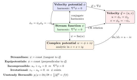
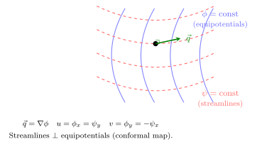
Velocity potential and stream function. For an irrotational incompressible 2D flow, there exists a velocity potential $\phi(x,y)$ with $\vec q = \nabla\phi$, i.e. $u=\phi_x,\;v=\phi_y$. Incompressibility ($\nabla\cdot\vec q=0$) forces $\phi$ to be harmonic: $\nabla^2\phi=\phi_{xx}+\phi_{yy}=0$. The conjugate harmonic $\psi$ (the stream function) satisfies the Cauchy–Riemann relations $u=\psi_y,\;v=-\psi_x$. Streamlines are $\psi=\text{const}$ and are everywhere perpendicular to the equipotentials $\phi=\text{const}$. The complex potential $w=\phi+i\psi$ is analytic in $z=x+iy$, and the complex velocity is $dw/dz=u-iv$.

Sign note. Some authors write $\vec q=-\nabla\phi$. The 2017 and 2016 UPSC solutions use this convention; the 2018, 2020, 2021 solutions use $\vec q=+\nabla\phi$. Either is acceptable — state it clearly at the start of every answer.

Testing motion possibility and finding $\psi$. A velocity potential $\phi$ represents a possible (incompressible irrotational) flow iff $\nabla^2\phi=0$. To find $\psi$: integrate $\partial\psi/\partial y=u$ w.r.t. $y$ to get $\psi=\int u\,dy+g(x)$; then differentiate and match $-\partial\psi/\partial x=v$ to determine $g(x)$.

Streamlines in 3D and special flows. Streamlines satisfy the ODE $dx/u=dy/v=dz/w$; integrate pairwise to find two independent first integrals. Key building blocks: uniform flow ($\phi=Ux$, streamlines horizontal); source/sink ($\phi=m\ln r$ in 2D, $\phi=-m/r$ in 3D); point vortex ($\phi=\Gamma\theta/2\pi$, streamlines = concentric circles, multi-valued); doublet/dipole in 3D ($\phi=-M\cos\theta/r^2$, streamlines $\sin^2\theta/r=\text{const}$). Unsteady irrotational flow satisfies Bernoulli’s equation: $p/\rho+\partial\phi/\partial t+\tfrac12|\vec q|^2=f(t)$, with $f(t)=p_\infty/\rho$ when the fluid is at rest at infinity.

Question Archetypes

Five patterns cover every potential flow question in the corpus.

potential-stream-function (5 question(s); 2017, 2018, 2020, 2021, 2022)

Recognition Cues

• “Find the stream function $\psi$” given a velocity potential $\phi$ — directly apply Cauchy–Riemann.
• “Show the motion is possible; find the velocity potential; find streamlines” — verify $\nabla^2\phi=0$ or $\nabla\cdot\vec q=0$, then integrate $\nabla\phi=\vec q$ to recover $\phi$.
• Velocity field given explicitly; you must integrate.

Solution Template

Given $\phi$, find $u,v,\psi$:

1. Compute $u=\phi_x,\;v=\phi_y$.
2. Check $\nabla^2\phi=u_x+v_y=0$ — if yes, “possible flow.”
3. Integrate $\psi_y=u$ w.r.t. $y$: $\psi=\int u\,dy+g(x)$.
4. Differentiate: $\psi_x=-v$. Determine $g'(x)$, hence $g(x)$. Write $\psi$.

Given $\vec q=(u,v,w)$, verify and find $\phi$:

1. Check $\nabla\cdot\vec q=u_x+v_y+w_z=0$.
2. Integrate $u=-\phi_x$ (or $+\phi_x$) to get $\phi$ up to a function of the remaining variables; match with $v,w$.
3. Find streamlines from $dx/u=dy/v=dz/w$.

Worked Example(s)

2018 Paper 2, 2018-P2-Q8b (15 marks)

For $\phi=x^2y-xy^2+\tfrac13(x^3-y^3)$, find velocity components, stream function, and check whether $\phi$ represents a possible flow.

Velocity. $u=\phi_x=2xy-y^2+x^2$; $v=\phi_y=x^2-2xy-y^2$.

Possibility check. $u_x=2x+2y$; $v_y=-2x-2y$; $\nabla^2\phi=u_x+v_y=0$. Possible flow.

Stream function. Integrate $\psi_y=u=x^2+2xy-y^2$: $\psi=x^2y+xy^2-\frac{y^3}{3}+g(x).$ Match $\psi_x=-v=-(x^2-2xy-y^2)$: $2xy+y^2+g'(x)=-x^2+2xy+y^2\;\Longrightarrow\;g'(x)=-x^2\;\Longrightarrow\;g=-\tfrac{x^3}{3}.$ $\boxed{\;\psi=x^2y+xy^2-\tfrac13(x^3+y^3).\;}$

2020 Paper 2, 2020-P2-Q7c (15 marks)

Velocity potential $\phi=xy+x^2-y^2$. Find the stream function.

Velocity. $u=\phi_x=y+2x$; $v=\phi_y=x-2y$. Check: $u_x+v_y=2+(-2)=0$ ✓.

Stream function. Integrate $\psi_y=u=2x+y$: $\psi=2xy+y^2/2+g(x)$. Match $\psi_x=-v=2y-x$: $2y+g'(x)=2y-x\;\Longrightarrow\;g'(x)=-x\;\Longrightarrow\;g=-x^2/2.$ $\boxed{\;\psi=2xy+\tfrac12(y^2-x^2)+C.\;}$

2021 Paper 2, 2021-P2-Q7c (20 marks)

Show $\vec q=\lambda(-y,x)/(x^2+y^2)$ is a possible incompressible flow. Find streamlines; is motion potential; find $\phi$.

Incompressibility. $u=-\lambda y/r^2$, $v=\lambda x/r^2$ where $r^2=x^2+y^2$. $u_x=\frac{2\lambda xy}{r^4},\quad v_y=\frac{-2\lambda xy}{r^4};\quad\nabla\cdot\vec q=0.\ \checkmark$

Streamlines. $dx/(-y)=dy/x\;\Rightarrow\;x\,dx+y\,dy=0\;\Rightarrow\;x^2+y^2=C$. Concentric circles.

Irrotationality. $\omega_z=v_x-u_y=\lambda(y^2-x^2)/r^4-\lambda(y^2-x^2)/r^4=0$. Irrotational except at origin.

Velocity potential. $\nabla(\lambda\arctan(y/x))=\lambda(-y/r^2,\,x/r^2)=\vec q$. $\boxed{\;\phi=\lambda\arctan(y/x)=\lambda\theta\quad(\text{multi-valued: point vortex}).\;}$

2017 Paper 2, 2017-P2-Q8c (15 marks)

Velocity $\vec q=(3xz/r^5,\,3yz/r^5,\,(3z^2-r^2)/r^5)$. Show motion possible, potential is $z/r^3$, find streamlines.

Incompressibility ($\nabla\cdot\vec q=0$). Compute $u_x+v_y+w_z$; use $x^2+y^2=r^2-z^2$ to collapse the terms: $\nabla\cdot\vec q=\frac{10z}{r^5}-\frac{15z(r^2-z^2)+15z^3-5zr^2}{r^7}=\frac{10z}{r^5}-\frac{10z}{r^5}=0.\ \checkmark$

Velocity potential (convention $\vec q=-\nabla\phi$). Verify $\phi=z/r^3$: $-\phi_x=3xz/r^5=u,\quad-\phi_y=3yz/r^5=v,\quad-\phi_z=(3z^2-r^2)/r^5=w.\ \checkmark$

Streamlines. From $dx/x=dy/y$: meridian planes $y/x=C_1$. In each plane, Stokes stream function $\psi=\rho^2/r^3$ (with $\rho=\sqrt{x^2+y^2}$) gives: $\boxed{\;\frac{y}{x}=C_1,\qquad\frac{x^2+y^2}{(x^2+y^2+z^2)^{3/2}}=C_2.\;}$ (Classical doublet/dipole streamlines — $\sin^2\theta/r=C_2$ in spherical coordinates.)

2022 Paper 2, 2022-P2-Q5e (10 marks)

Spherical velocity: $v_r=2Mr^{-3}\cos\theta$, $v_\theta=Mr^{-3}\sin\theta$ (corrected exponent). Show potential flow; find $\phi$ and streamlines.

Irrotationality (spherical $\psi$-component of curl): $(\nabla\times\vec v)_\phi=\frac{1}{r}\!\left[\frac{\partial(rv_\theta)}{\partial r}-\frac{\partial v_r}{\partial\theta}\right]=\frac1r\!\left[-2Mr^{-3}\sin\theta-(-2Mr^{-3}\sin\theta)\right]=0.\ \checkmark$

Velocity potential. $v_r=\partial\phi/\partial r=2M\cos\theta/r^3$; integrate: $\phi=-M\cos\theta/r^2+g(\theta)$. Match $v_\theta=(1/r)\partial\phi/\partial\theta=M\sin\theta/r^3$: $g'(\theta)=0$. $\boxed{\;\phi=-\frac{M\cos\theta}{r^2}\quad(\text{3D doublet/dipole}).\;}$

Streamlines via Stokes stream function: $\psi=M\sin^2\theta/r$, so streamlines are $\sin^2\theta/r=\text{const}$.

Common Traps

• Possible flow = $\nabla^2\phi=0$ (not just “irrotational”). A velocity potential automatically implies irrotational; the remaining condition is harmonicity, which is equivalent to incompressibility.
• Stream function sign convention $u=\psi_y,\;v=-\psi_x$ (not $u=-\psi_y$). A sign slip flips $\psi$ and gives the wrong conjugate.
• The arbitrary constant $C$ in $\psi$ is genuine (stream functions are defined up to an additive constant); don’t set it to zero unless a boundary condition requires it.
• In 3D, streamlines require the Stokes stream function (in spherical or cylindrical coords), not naive integration of $dz/w$. The 2017 doublet streamlines need $\psi=\rho^2/r^3$, not $y/x=\text{const}$ alone.

streamlines-from-potential (2 question(s); 2014, 2024)

Recognition Cues

• $\phi$ is given; you must find the streamlines (no $\psi$ computation required in full — just identify level curves).
• The potential is often a logarithm or simple polynomial; the streamlines are geometric objects (circles, planes, ruled surfaces).

Solution Template

1. Compute $\vec q=\nabla\phi$ to get $u,v$ (2D) or $u,v,w$ (3D).
2. 2D: use the complex potential $w=\phi+i\psi$; read $\psi=\operatorname{Im}(w)$; streamlines are $\psi=\text{const}$.
3. 3D: write the streamline ODEs $dx/u=dy/v=dz/w$; integrate pairwise to get two independent first integrals $f(x,y,z)=C_1$ and $g(x,y,z)=C_2$.
4. Identify the geometric shape of the level curves (circles, planes, hyperboloids, etc.).

Worked Example(s)

2014 Paper 2, 2014-P2-Q7c (20 marks)

$\phi=\tfrac12\log\!\left[\tfrac{(x+a)^2+y^2}{(x-a)^2+y^2}\right]$. Determine the streamlines.

Identify the flow. Write $\phi=\ln r_1-\ln r_2$ where $r_{1,2}=\sqrt{(x\pm a)^2+y^2}$. This is a source at $(-a,0)$ and sink at $(a,0)$ of unit strength.

Complex potential. $w=\log(z+a)-\log(z-a)=\log\!\dfrac{z+a}{z-a}$.

Stream function. $\psi=\operatorname{Im}(w)=\arg\dfrac{z+a}{z-a}=\theta_1-\theta_2$, where $\theta_1,\theta_2$ are the angles from $(\mp a,0)$ to $(x,y)$.

Streamlines $\psi=k$. Setting $\theta_1-\theta_2=k$ and using $\tan(\theta_1-\theta_2)=-2ay/(x^2+y^2-a^2)$: $x^2+y^2+\frac{2a}{k}y-a^2=0\;\Longrightarrow\;x^2+\!\left(y+\frac ak\right)^2=\frac{a^2(k^2+1)}{k^2}.$

$\boxed{\;\text{Streamlines are circles centred on the }y\text{-axis, each passing through }(\pm a,0).\;}$

(Inscribed-angle theorem: constant subtended angle ⟺ circular arc through the chord endpoints.)

2024 Paper 2, 2024-P2-Q5e (10 marks)

$\phi=\tfrac12(x^2+y^2-2z^2)$. Determine the streamlines.

Velocity. $u=x$, $v=y$, $w=-2z$. (Check: $\nabla^2\phi=1+1-2=0$ ✓.)

Streamline ODEs. $dx/x=dy/y=dz/(-2z)$.

Pair 1 ($dx/x=dy/y$): $y/x=C_1$.

Pair 2 ($dx/x=dz/(-2z)$): $2\ln|x|+\ln|z|=\text{const}$, i.e. $x^2z=C_2$.

$\boxed{\;\frac{y}{x}=C_1\quad\text{and}\quad x^2z=C_2.\;}$

(Intersections of meridian planes $y=C_1 x$ with hyperbolic surfaces $z=C_2/x^2$. These are not circles — check $\nabla^2\phi=0$ to confirm this is genuinely a potential flow.)

Common Traps

• 3D streamlines are curves (two equations), not surfaces. Reporting only one first integral is incomplete.
• The inscribed-angle construction for the source-sink potential (2014) converts the algebra into a familiar geometric statement; derive it, don’t just quote it.
• Don’t confuse streamlines ($\psi=\text{const}$) with equipotentials ($\phi=\text{const}$) — in the 2024 problem, $\phi=\text{const}$ gives hyperboloids $x^2+y^2-2z^2=\text{const}$, which are the equipotentials, not the streamlines.

complex-potential-analysis (1 question(s); 2021)

Recognition Cues

• A complex function $w(z)$ is given as the “complex potential” (or “complex velocity potential”); you must extract the real and imaginary parts and identify the resulting curves.
• The question asks for streamlines, equipotentials, velocity, and singularities.

Solution Template

1. Write $w=\phi+i\psi$ by expressing $w$ in terms of $z=x+iy$.
2. For $w$ involving $\log$ or $\arctan$: use $\log(Re^{i\Theta})=\ln R+i\Theta$ to identify $\phi=\Theta/2$ or $\phi=\ln R$, etc.
3. Streamlines: set $\psi=\text{const}$ and identify the geometric locus (often a circle or line).
4. Equipotentials: set $\phi=\text{const}$ — these are the orthogonal family.
5. Velocity: $dw/dz=u-iv$; compute this derivative.
6. Singularities: where $dw/dz$ is undefined or where $w$ has a branch point.

Worked Example(s)

2021 Paper 2, 2021-P2-Q8c (20 marks)

Complex potential $w=\tan^{-1}z$. Show streamlines and equipotential curves are circles; find velocity; check singularities at $z=\pm i$.

Logarithmic form. $w=\tan^{-1}z=\dfrac{1}{2i}\ln\!\dfrac{1+iz}{1-iz}$.

Write $\dfrac{1+iz}{1-iz}=Re^{i\Theta}$. Since $\operatorname{Re}(w)=\Theta/2=\phi$ and $\operatorname{Im}(w)=-\ln R/2=\psi$.

Compute: $R=\dfrac{|1+iz|}{|1-iz|}=\dfrac{\sqrt{(1-y)^2+x^2}}{\sqrt{(1+y)^2+x^2}}$.

Streamlines ($\psi=$ const, i.e. $R=$ const): $\frac{x^2+(1-y)^2}{x^2+(1+y)^2}=k\;\Longrightarrow\;x^2+\!\left(y-\frac{1+k}{1-k}\right)^2=\frac{4k}{(1-k)^2}.$ These are circles with centres on the $y$-axis passing through $(0,\pm1)$.

Equipotentials ($\phi=$ const, $\Theta=$ const): the angle subtended at $(x,y)$ by the segment $[-i,+i]$ is constant. By the inscribed-angle theorem, equipotentials are also circles through $(0,\pm1)$, orthogonal to the streamlines.

Velocity. $dw/dz=\dfrac{1}{1+z^2}$.

Singularities. $1+z^2=0\Rightarrow z=\pm i$: logarithmic branch points of $w$; velocity diverges there.

$\boxed{\;\text{Both families are circles through }(0,\pm1);\quad V=1/(1+z^2);\quad\text{branch points at }z=\pm i.\;}$

Common Traps

• The denominator factor $(1-k)$ in the streamline circle equation vanishes at $k=1$ (the $x$-axis, a degenerate streamline); handle this limiting case separately.
• The inscribed-angle theorem applies to both families: $\Theta=\text{const}$ and $\ln R=\text{const}$ each describe a Steiner circle pencil through the two branch points $\pm i$.

potential-boundary-value (1 question(s); 2016)

Recognition Cues

• Liquid fills the region between two surfaces (spheres, cylinders); each boundary moves with a specified velocity.
• You must find $\phi$ matching the normal-velocity condition $(-\nabla\phi)\cdot\hat n=\mathbf W\cdot\hat n$ on each boundary.

Solution Template

1. Write $\phi$ as a linear combination of the elementary harmonic functions appropriate to the geometry (e.g. $x,\;x/r^3$ for each Cartesian direction in 3D spherical geometry).
2. Compute the normal velocity $\partial\phi/\partial r$ on each shell.
3. Match to the specified boundary velocity component in the normal direction — this gives one equation per shell per direction.
4. Solve the linear system for the coefficients.
5. Compute $\vec q=-\nabla\phi$ to find the velocity at any interior point.

Worked Example(s)

2016 Paper 2, 2016-P2-Q7b (20 marks)

Liquid between concentric spheres $r=a$ (moving $U\hat i$) and $r=b$ (moving $V\hat j$). Show the potential is $\phi=\bigl[a^3U(1+\tfrac12 b^3r^{-3})x-b^3V(1+\tfrac12 a^3r^{-3})y\bigr]/(b^3-a^3)$ and find the velocity.

Harmonic ansatz. The natural harmonics linear in a direction are $x$ and $x/r^3$ (each satisfies $\nabla^2=0$). Take $\phi=(Ax+Bx/r^3)+(Cy+Ey/r^3)$, with the $x$-group carrying the inner-sphere $U$-condition and the $y$-group the outer-sphere $V$-condition.

Boundary conditions (normal velocity on each sphere, $\vec q=-\nabla\phi$, $\hat n=\mathbf r/r$):

• Inner $r=a$, normal velocity $= U(x/a)$: gives two equations for $A,B$.
• Outer $r=b$, normal velocity $= V(y/b)$: gives two equations for $C,E$.

Coefficients: $A=\frac{a^3U}{b^3-a^3},\quad B=\frac{a^3b^3U}{2(b^3-a^3)},\quad C=\frac{-b^3V}{b^3-a^3},\quad E=\frac{-a^3b^3V}{2(b^3-a^3)}.$

Substituting gives the stated $\phi$. $\blacksquare$

Velocity. Differentiating $\phi$ using $\partial_x(x/r^3)=r^{-3}-3x^2r^{-5}$ etc.: $\boxed{\;\vec q=\frac{-a^3U\hat i+b^3V\hat j}{b^3-a^3}+\frac{a^3b^3}{2r^3(b^3-a^3)}\!\left[\frac{3(\mathbf d\cdot\hat r)\hat r\cdot r}{r}-\mathbf d\right],\quad\mathbf d=U\hat i-V\hat j.\;}$

Common Traps

• Normal-velocity BC: $(-\nabla\phi)\cdot\hat n = \mathbf W\cdot\hat n$, not $(-\nabla\phi)\cdot\mathbf W$. Use $\hat n=\mathbf r/r$ and project $\mathbf W$ onto $\hat n$ explicitly.
• The $x$- and $y$-motions decouple: solve two $2\times2$ systems, not one $4\times4$.
• Differentiating $x/r^3$ yields cross terms ($\partial_y(x/r^3)=-3xy/r^5$), so $u$ depends on $V$ and $w\neq0$ even though the shells move in the $xy$-plane.

unsteady-bernoulli (1 question(s); 2019)

Recognition Cues

• A sphere (or bubble) of time-varying radius $R(t)$ is embedded in fluid at rest at infinity; find the surface pressure.
• The phrase “vibrating sphere” or “pulsating bubble” signals this archetype.
• The unsteady Bernoulli term $\partial\phi/\partial t$ is the distinguishing feature.

Solution Template

1. Write $\phi=-F(t)/r$ (radial harmonic for incompressible irrotational flow at infinity, decaying). From $u=\partial\phi/\partial r=F/r^2$ and the BC $u(R,t)=\dot R$: determine $F(t)=R^2\dot R$.
2. Compute $\partial\phi/\partial t$ at $r=R$; compute $u^2$ at $r=R$.
3. Apply unsteady Bernoulli: $p=\Pi-\rho(\partial\phi/\partial t+\tfrac12 u^2)$ (where $\Pi$ = pressure at infinity).
4. Substitute and simplify. Common result: $p_R=\Pi+\rho(R\ddot R+\tfrac32\dot R^2)$.
5. If required, rewrite using $d^2(R^2)/dt^2=2\dot R^2+2R\ddot R$ to match the stated form.

Worked Example(s)

2019 Paper 2, 2019-P2-Q8b (15 marks)

Sphere radius $R(t)$ vibrates radially in infinite incompressible fluid. Establish the surface pressure $\Pi+\tfrac12\rho\{d^2(R^2)/dt^2+(\dot R)^2\}$.

Step 1 — Velocity potential. Radial symmetry: $\phi=-F(t)/r$, $u=F/r^2$. BC at $r=R$: $F=R^2\dot R$. So $\phi=-R^2\dot R/r$.

Step 2 — Terms at $r=R$. $\left.\frac{\partial\phi}{\partial t}\right|_R=-\frac{d}{dt}(R^2\dot R)=-(2R\dot R^2+R^2\ddot R),\qquad u^2|_R=\dot R^2.$

Step 3 — Unsteady Bernoulli. $p_R=\Pi-\rho\!\left[-(2R\dot R^2+R^2\ddot R)+\tfrac12\dot R^2\right]=\Pi+\rho\!\left(R\ddot R+\tfrac32\dot R^2\right).$

Step 4 — Reconcile with printed form. $\tfrac12\rho\{d^2(R^2)/dt^2+\dot R^2\}=\tfrac12\rho\{(2\dot R^2+2R\ddot R)+\dot R^2\}=\rho(R\ddot R+\tfrac32\dot R^2)$. ✓

$\boxed{\;p_R=\Pi+\tfrac12\rho\!\left\{\tfrac{d^2(R^2)}{dt^2}+\!\left(\tfrac{dR}{dt}\right)^2\right\}.\;}\quad\blacksquare$

Common Traps

• Must use unsteady Bernoulli (keep $\partial\phi/\partial t$); the quasi-steady form drops this term entirely and gives a wrong answer.
• The $\tfrac32\dot R^2$ arises as $+2\dot R^2$ (from $\partial\phi/\partial t$) minus $\tfrac12\dot R^2$ (from the $-\tfrac12u^2$ sign). Tracking the sign of $u^2$ in Bernoulli ($-\tfrac12u^2$ on the RHS or $+\tfrac12u^2$ on the LHS) is the main source of errors.
• The printed UPSC notation $\dfrac{d^2R^2}{dt^2}$ means $\dfrac{d^2(R^2)}{dt^2}=2\dot R^2+2R\ddot R$, not $\left(\dfrac{d^2R}{dt^2}\right)^2$ or $\dfrac{d^2R}{dt^2}$.

Marks-Aware Writing

10-mark questions (2022-Q5e, 2024-Q5e): One to two sentences of setup (state $\phi$ or the flow type), then execute the algorithm. For streamlines: write the two ODEs, integrate in pairs, box the result. No lengthy preamble.

15-mark questions (2017, 2018, 2019, 2020): Three to four clear steps. For the stream function: verify possibility ($\nabla^2\phi=0$), then integrate step by step. For unsteady Bernoulli: label Steps 1–3 (potential, evaluate at $r=R$, Bernoulli). The verification step at the end earns the final method marks.

20-mark questions (2014, 2016, 2021-Q7c, 2021-Q8c): Full proof format. For boundary-value problems: state the harmonic ansatz, write both BCs, solve the coefficient system, then differentiate for velocity. For complex potentials: extract $\phi,\psi$ explicitly, then show each geometric claim separately (streamlines circles, equipotentials circles, velocity, singularities).

Practice Set