Surface integrals; flux

At a Glance

• Frequency: 1 sub-part across 1 of 14 years (2026)
• Priority tier: T4 by the frequency rule (first headline appearance is 2026) — but work this chapter before P1-VA-15 and P1-VA-16, which depend on it
• Marks (count): 10 (1, in 2026); as a supporting topic it carries part of nine further questions worth 10–20 each
• Average solve time: ~10 min standalone; it is the inner 5–8 minutes of most Gauss and Stokes questions
• Difficulty mix: easy standalone, medium-to-hard inside a theorem verification
• Section: B | Dominant type: computation

Why This Chapter Matters

This is the atom the syllabus hides. For fourteen years UPSC never once made the surface integral the subject of a question — it was always the machinery inside something bigger: verify Gauss, verify Stokes, evaluate a flux “hence”. Then in 2026 it appeared on its own, in Q5(e), in the compulsory question, where no amount of question choice could route around it.

That history is exactly why it is dangerous. A candidate who has only ever met $\iint_S \vec F\cdot\hat n\,dS$ inside the divergence theorem has learned it as a step, not as an object — and when the step becomes the question, there is nothing to fall back on.

There is a second, larger reason. Gauss’s theorem and Stokes’ theorem are both machines for converting surface integrals into something else. Between them they account for 18 sub-parts across 2013–2025 — more than any other pair of atoms in Vector Analysis. You cannot verify a theorem whose two sides you cannot each compute. Every mark in P1-VA-15 and P1-VA-16 sits on top of this chapter. Study it first, and those two become bookkeeping; skip it, and they become guesswork.

Minimum Theory

The two integrals. For a scalar field $f$ and a vector field $\vec F$ over a surface $S$: $\iint_S f\,dS \qquad\text{(scalar surface integral)},\qquad \iint_S \vec F\cdot\hat n\,dS \qquad\text{(flux of }\vec F\text{ through }S).$ Only the second appears in UPSC Paper I with any regularity. $\hat n$ is a unit normal to $S$; $dS$ is the element of area.

Orientation is a choice you must state. A two-sided surface has two unit normals, $\pm\hat n$, and the flux changes sign with the choice. For a closed surface the convention is the outward normal. For an open surface the paper must tell you — and if it does not, say which one you are taking. That single sentence has been worth a mark.

Route 1 — Projection onto a coordinate plane (the workhorse)

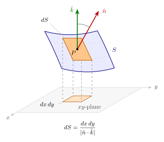
If $S$ projects one-to-one onto a region $R$ in the $xy$-plane, then $\boxed{\,dS=\frac{dx\,dy}{|\hat n\cdot\hat k|}\,}\qquad\Longrightarrow\qquad \iint_S \vec F\cdot\hat n\,dS=\iint_R \frac{\vec F\cdot\hat n}{|\hat n\cdot\hat k|}\,dx\,dy .$

The factor $1/|\hat n\cdot\hat k|$ is the “un-squashing” factor: a tilted patch casts a smaller shadow than its own area, and the more tilted it is, the bigger the correction. When $\hat n\perp\hat k$ the surface is vertical, its shadow has zero area, and the formula breaks — which is precisely the case where the projection is not one-to-one and you must project onto $yz$ or $zx$ instead.

Two conditions to check before using it, both creditable:

1. the projection is one-to-one (a sphere is not — split it into hemispheres);
2. $\hat n\cdot\hat k\neq0$ on $S$.

Route 2 — Surface given as a graph $z=g(x,y)$ (the fastest form)

This is Route 1 with the algebra already done, and it is the form to memorise: $\boxed{\,\hat n\,dS=\bigl(-g_x,\,-g_y,\,1\bigr)\,dx\,dy\,}\qquad\text{(upward normal)},\qquad dS=\sqrt{1+g_x^2+g_y^2}\;dx\,dy .$

It is worth seeing why, because it makes the $1/|\hat n\cdot\hat k|$ factor obvious. Writing $S$ as $z-g(x,y)=0$, the gradient gives $\hat n=\dfrac{(-g_x,-g_y,1)}{\sqrt{1+g_x^2+g_y^2}}$, so $\hat n\cdot\hat k=\dfrac{1}{\sqrt{1+g_x^2+g_y^2}}$ and the radical cancels when $\hat n$ is multiplied by $dS$. The radical never has to be computed. Candidates who work with $\hat n$ and $dS$ separately spend two minutes on a square root that was always going to cancel.

For the downward normal, negate: $\hat n\,dS=(g_x,\,g_y,\,-1)\,dx\,dy$.

Route 3 — Parametric surface

If $\vec r=\vec r(u,v)$ over a parameter domain $D$: $dS=\left|\vec r_u\times\vec r_v\right|du\,dv,\qquad \hat n\,dS=\pm\left(\vec r_u\times\vec r_v\right)du\,dv,$ the sign fixed by the required orientation. Use this when the surface is naturally parametrised (sphere, cone, cylinder) and awkward as a graph.

The three standard surfaces — know these cold

The sphere identity is the biggest time-saver in the chapter. On $x^2+y^2+z^2=a^2$ the outward normal is radial, so $\vec F\cdot\hat n=\vec F\cdot\vec r/a$ — and if $\vec F=\vec r$ this collapses to the constant $a$, giving $\iint_S\vec r\cdot\hat n\,dS=a\cdot4\pi a^2=4\pi a^3$ with no integration at all. (Sanity check via the divergence theorem: $\nabla\cdot\vec r=3$, so the flux is $3\times\tfrac43\pi a^3=4\pi a^3$. ✓)

Question Archetypes

Four patterns cover everything this atom has been asked, in fourteen years, as headline or support.

Where these are filed, and why it matters. Only plane-patch is catalogued as a P1-VA-14 archetype, because 2026 Q5(e) is the one question where the surface integral itself was the headline. The other three describe questions filed under P1-VA-15 (Gauss) or P1-VA-16 (Stokes) — there the theorem is the headline and the surface integral is the machinery inside it. That filing is precisely the problem this chapter exists to fix: the skill is identical in all four cases, and a candidate who only ever meets it under someone else’s heading never learns it as a technique in its own right. Work all four here; you will meet the last three again, in disguise, in the Gauss and Stokes chapters.

plane-patch (2026 Paper I Q5(e); the 2026 headline appearance)

Recognition Cues

• $S$ is a single plane, $ax+by+cz=d$, “bounded by” four coordinate planes or lines.
• The integrand is $\vec F\cdot\hat n$ or $(\nabla\times\vec F)\cdot\hat n$ where the field is linear, so the integrand is constant.

Solution Template

1. Compute $\hat n$ from the plane’s coefficients. It is constant — say so.
2. State the orientation you are taking if the paper does not.
3. Compute the (constant) integrand.
4. $dS=\dfrac{dx\,dy}{|\hat n\cdot\hat k|}$; the integral is (constant) $\times$ (area of the projected region).
5. Cross-check with Stokes if a curl is involved.

Worked Example

2026 Paper 1, 2026-P1-Q5e (10 marks)

$\vec F=(2x+3y)\hat i-4z\hat j-5x\hat k$; $S$ is $2x+4y+4z=5$ bounded by $x=0$, $x=2$, $y=0$, $y=3$. Evaluate $\iint_S(\nabla\times\vec F)\cdot\hat n\,dS$.

$\nabla\times\vec F=\bigl(0-(-4),\;0-(-5),\;0-3\bigr)=4\hat i+5\hat j-3\hat k\quad\text{(constant)}.$

The plane $2x+4y+4z=5$ has $\nabla\phi=(2,4,4)$, $|\nabla\phi|=6$. The paper does not prescribe an orientation; take the upward normal (the other choice reverses the sign): $\hat n=\tfrac13\hat i+\tfrac23\hat j+\tfrac23\hat k,\qquad \hat n\cdot\hat k=\tfrac23 .$

$(\nabla\times\vec F)\cdot\hat n=\frac{8+20-12}{6}=\frac{8}{3},\qquad dS=\frac{dx\,dy}{2/3}=\frac32\,dx\,dy .$

The patch projects one-to-one onto the rectangle $0\le x\le2$, $0\le y\le3$, of area $6$: $\iint_S(\nabla\times\vec F)\cdot\hat n\,dS=\frac83\cdot\frac32\cdot 6=\boxed{\;24\;}$

Common Traps

• Orientation. Unspecified here. Two marks’ worth of difference and one line to protect: name your normal.
• Do not integrate $\hat n$ — on a plane it is constant and comes straight out of the integral.
• The four “bounding surfaces” are planes parallel to the $z$-axis; they cut the plane in four lines and the patch projects exactly onto the rectangle. Say that the projection is one-to-one.

graph-projection (2020-P1-Q7a; the archetype to drill)

Recognition Cues

• $S$ is given explicitly as $z=g(x,y)$ over a rectangle or simple region — often a parabolic sheet, “part of the cylinder $z=1-x^2$”.
• The word “cylinder” here means a sheet, not a closed tube. Read the bounds.

Solution Template

1. Write $\hat n\,dS=(-g_x,-g_y,1)\,dx\,dy$ for the upward normal. Do not compute $\sqrt{1+g_x^2+g_y^2}$.
2. Substitute $z=g(x,y)$ into the field.
3. Dot, then integrate over the projected region.
4. Exploit odd symmetry before integrating.

Worked Example

2020 Paper 1, 2020-P1-Q7a (20 marks)

Verify Stokes’ theorem for $\vec F=xy\,\hat i+yz\,\hat j+xz\,\hat k$ on $S$: part of $z=1-x^2$, $0\le x\le1$, $-2\le y\le2$, oriented upwards.

$\nabla\times\vec F=(-y,\,-z,\,-x).$

With $g=1-x^2$: $g_x=-2x$, $g_y=0$, so $\hat n\,dS=(2x,\,0,\,1)\,dx\,dy$ and $(\nabla\times\vec F)\cdot\hat n\,dS=\bigl[-y(2x)+(-z)(0)+(-x)(1)\bigr]dx\,dy=(-2xy-x)\,dx\,dy .$

Note the $z$-component of $\hat n\,dS$ multiplied $-z$, so $z$ never had to be substituted. Over $-2\le y\le2$ the term $-2xy$ is odd in $y$ and integrates to zero: $\iint_R(-2xy-x)\,dA=\int_0^1\!\!\int_{-2}^{2}(-x)\,dy\,dx=\int_0^1(-4x)\,dx=\boxed{\;-2\;}$

and the boundary circulation gives $-2$ as well, verifying the theorem.

Common Traps

• Computing $\hat n$ and $dS$ separately and carrying $\sqrt{1+4x^2}$ through the whole problem. It cancels. Use $\hat n\,dS$ as one object.
• Forgetting that “oriented upwards” fixes the sign of $(-g_x,-g_y,1)$, and that the boundary must then be traversed by the right-hand rule.
• Missing the odd-in-$y$ symmetry and grinding out a term that is zero.

closed-surface (2022-P1-Q8c, 2021-P1-Q7a, 2023-P1-Q6c)

Recognition Cues

• $S$ is the whole boundary of a solid: a cube, a cylinder with its lids, a sphere.
• Usually phrased “verify the divergence theorem”, which means compute both sides independently.

Solution Template

1. Volume side: $\nabla\cdot\vec F$, then $\iiint_V(\nabla\cdot\vec F)\,dV$ in whatever coordinates suit the solid.
2. Surface side: split into faces. On each face, $\hat n$ is one of $\pm\hat i,\pm\hat j,\pm\hat k$ (flat faces) or radial/lateral (curved). Always outward.
3. Identify the faces that contribute zero before integrating — that is where the time is saved.
4. Sum and state equality.

Worked Example

2022 Paper 1, 2022-P1-Q8c (15 marks)

Verify Gauss’s divergence theorem for $\vec F=x\hat i-y\hat j+(z^2-1)\hat k$ over the cylinder $x^2+y^2=4$, $0\le z\le1$.

Volume side. $\nabla\cdot\vec F=1-1+2z=2z$, so $\iiint_V 2z\,dV=\left(\int_0^1 2z\,dz\right)\times(\text{cross-section area }4\pi)=1\cdot4\pi=4\pi .$

Surface side, three pieces:

• Bottom $z=0$, $\hat n=-\hat k$: $\vec F\cdot\hat n=-(z^2-1)\big|_{z=0}=1$, contributing $1\times4\pi=4\pi$.
• Top $z=1$, $\hat n=\hat k$: $\vec F\cdot\hat n=z^2-1=0$. Contributes nothing — spot this before integrating.
• Lateral $\hat n=\tfrac12(x,y,0)$: $\vec F\cdot\hat n=\tfrac12(x^2-y^2)=2\cos2\phi$ on $x=2\cos\phi,\ y=2\sin\phi$, and $dS=2\,d\phi\,dz$. Then $\int_0^{2\pi}\cos2\phi\,d\phi=0$, so this contributes nothing either.

Total $=\boxed{\;4\pi\;}$, agreeing with the volume side. ✓

Common Traps

• Using an inward normal on one face. On a closed surface every normal is outward; on the bottom face that means $-\hat k$, and the sign flip is the commonest single error in this archetype.
• Grinding the lateral integral when $\cos2\phi$ averages to zero over a full turn.
• On a hemisphere (2023-P1-Q6c) the surface is not closed: you must add the flat disk $z=0$ to apply Gauss, then subtract the disk’s own contribution at the end.

open-surface-cap (2020-P1-Q8b, 2016-P1-Q8b)

Recognition Cues

• $S$ is a hemisphere, cap or open sheet with a boundary curve, and the integrand is a curl.
• $\iint_S(\nabla\times\vec F)\cdot\hat n\,dS$ over a cap whose rim is a simple circle.

Solution Template

1. Recognise the integrand as a curl. Identify the boundary curve $C$.
2. Apply Stokes: $\iint_S(\nabla\times\vec F)\cdot\hat n\,dS=\oint_C\vec F\cdot d\vec r$.
3. Orient $C$ by the right-hand rule against the chosen $\hat n$.
4. Evaluate the (usually much easier) line integral. Watch for an exact differential.

Worked Example

2020 Paper 1, 2020-P1-Q8b (15 marks)

Evaluate $\iint_S(\nabla\times\vec F)\cdot\hat n\,dS$ for $\vec F=y\hat i+(x-2xz)\hat j-xy\hat k$, $S$ the part of $x^2+y^2+z^2=a^2$ above the $xy$-plane.

Direct evaluation over the hemisphere is possible but slow. By Stokes the flux equals the circulation round the rim $C$: the circle $x^2+y^2=a^2$, $z=0$.

On $z=0$ the field reduces to $\vec F=y\hat i+x\hat j-xy\hat k$, and with $d\vec r=(dx,dy,0)$, $\vec F\cdot d\vec r=y\,dx+x\,dy=d(xy),$ an exact differential. Its integral round any closed curve vanishes: $\iint_S(\nabla\times\vec F)\cdot\hat n\,dS=\oint_C d(xy)=\boxed{\;0\;}$

(For the record, $\nabla\times\vec F=(x,\,y,\,-2z)$, and direct integration over the hemisphere confirms $0$.)

Common Traps

• Grinding the hemisphere directly when the rim integral is three lines. If the integrand is a curl and the surface has a rim, look at the rim first.
• Failing to notice $y\,dx+x\,dy=d(xy)$. Exact differentials round closed curves are free marks.
• Orientation: an upward $\hat n$ on the cap forces $C$ anticlockwise seen from above.

Common Traps (whole chapter)

1. Not stating the orientation. The single most reliable mark in this atom. If the paper is silent, write one sentence naming your normal — 2026 Q5(e) was silent.
2. Computing $\sqrt{1+g_x^2+g_y^2}$. On a graph surface it always cancels against $\hat n$. Use $\hat n\,dS=(-g_x,-g_y,1)\,dx\,dy$ as a single object.
3. Projecting a surface that does not project one-to-one. A full sphere must be split; a vertical face has $\hat n\cdot\hat k=0$ and must be projected onto a different plane.
4. Inward normals on a closed surface. Outward, always — and on the bottom face that is $-\hat k$.
5. Missing the free zeros. Faces where $\vec F\cdot\hat n$ vanishes identically, and $\phi$-integrals of $\cos2\phi$ or $\sin\phi$ over a full turn. Identify them before integrating and say why they vanish; it reads as fluency.
6. Treating a hemisphere as closed. It has a rim. Either close it with the disk (for Gauss) or use the rim (for Stokes).

What to Practise

In order:

1. 2026-P1-Q5e — the plane patch, and the only headline instance. Do it twice, once with each orientation, to see the sign flip.
2. 2020-P1-Q7a — the graph formula $\hat n\,dS=(-g_x,-g_y,1)\,dxdy$, which is the highest-yield single line in this chapter.
3. 2022-P1-Q8c — closed surface, face-by-face, with two faces contributing nothing.
4. 2020-P1-Q8b — when to abandon the surface and take the rim instead.
5. 2023-P1-Q6c — the hemisphere-plus-disk manoeuvre; the hardest of the six.

Then, and only then, work P1-VA-15 (Gauss) and P1-VA-16 (Stokes). Those two chapters assume everything above, and between them they are worth more marks than any other pair in Vector Analysis.